A program evaluation reports that a job-training program raised average earnings by $500. A city council member asks a different question: did the program make anyone worse off? The average cannot answer that question. We would see an average gain of $500 if every participant gained $500. We would see the same average if two thirds of the participants gained $1500 and one third lost $1500.
With data from a randomized experiment, cmrss() gives
the council member two numbers, both holding together with 95 percent
confidence: at least this many participants were made worse off, and at
most this many could have been. This vignette shows how to compute both
and how to read them.
What a randomized experiment can tell us about individual effects
Call each participant a unit. Each unit i has two potential outcomes: , the outcome it would have if treated, and , the outcome it would have if not treated. Its individual effect is . The unit was harmed if . We see only one of the two potential outcomes for each unit. So we never see any . We cannot say which units were harmed.
We can still learn how many units were harmed. Sort the n individual effects from smallest to largest, . Because treatment was assigned at random, we can test the hypothesis that the k-th smallest effect is at most some number c, written . We reject that hypothesis when the observed data would be unlikely, under random assignment, if were at most c. The largest c that we reject at the 5 percent level is a 95 percent lower confidence bound for .
cmrss() returns a lower bound for every k from 1 to
n. The bounds are built so that all n of them hold together with 95
percent confidence (see ?com_conf_quant_larger_cre). We may
therefore look through the whole list and pick out the bounds above 0.
Suppose the lower bound for
is above 0. The effects
are at least as large as
.
So, with 95 percent confidence, all
effects from
to
are above 0. At least
units have positive effects. cmrss() reports this count for
the smallest such k.
Counting harmed units with a minus sign
Lower bounds count units with positive effects. To count harmed units
we need to show that some effects are below 0. A lower bound cannot show
that. To count them, we multiply every outcome by -1 and analyze the new
outcome,
,
in place of
.
Each unit’s effect on
is
.
A harmed unit, with
,
therefore has a positive effect on
.
The count of units with positive effects on
is a count of harmed units. In cmrss() the change is a
minus sign in the formula: cmrss(-y ~ z, data = d).
When larger outcomes are worse, as with blood pressure or days absent, harm means . The analysis of y itself then counts harmed units.
A simulated program that harms some participants
We simulate an experiment in which we set every unit’s effect, so we can compare the answers with the truth. Of 200 units, 100 gain 2 points, 40 lose 3 points, and 60 are unaffected. Half the units are assigned to treatment at random.
set.seed(20261004)
n <- 200
y0 <- rnorm(n)
tau <- rep(0, n)
who <- sample(n)
tau[who[1:40]] <- -3     # harmed
tau[who[41:140]] <- 2    # helped
z <- sample(rep(c(1, 0), each = n / 2))
sim <- data.frame(z = z, y = ifelse(z == 1, y0 + tau, y0))
diff_means <- mean(sim$y[sim$z == 1]) - mean(sim$y[sim$z == 0])
The average effect is points. In this simulated experiment the treated group’s mean outcome exceeds the control group’s by 0.51 points. A researcher who reported only that difference would tell the council member the program helped. The difference says nothing about the 40 units the program harmed.
We ask the data two questions: how many units were helped, and how
many were harmed. We want both answers to hold together with 95 percent
confidence. The chance that at least one of two statements is wrong is
at most the sum of the two chances. So if we compute each at 97.5
percent confidence, both hold together with at least 95 percent
confidence. In cmrss() that is alpha = 0.025,
where alpha is one minus the confidence level. To keep this
page quick to build, each call below uses 1000 simulated random
assignments (nperm) and finds each bound to within 0.05
(tol). A real analysis should use the defaults of 10,000
assignments and 0.01.
helped <- cmrss(y ~ z, data = sim, set = "all", alpha = 0.025,
                nperm = nperm, tol = tol)
harmed <- cmrss(-y ~ z, data = sim, set = "all", alpha = 0.025,
                nperm = nperm, tol = tol)
helped
#> cmrss: completely randomized experiment, 200 units, 100 treated
#> Polynomial scores with parameters 2, 11, 66; 1000 simulated assignments
#> With 97.5 percent confidence, at least 18 of 200 units have effects on y above 0.
harmed
#> cmrss: completely randomized experiment, 200 units, 100 treated
#> Polynomial scores with parameters 2, 11, 66; 1000 simulated assignments
#> With 97.5 percent confidence, at least 7 of 200 units have effects on -y above 0.
n_harmed <- sum(harmed$bounds$lower > 0)
n_helped <- sum(helped$bounds$lower > 0)
With set = "all", cmrss() bounds the
effects of all 200 units, treated and control. It does so by bounding
the treated units and the control units separately, each at half of
alpha. The other choices, set = "treat" and
set = "control", bound one group at the full
alpha. Analyzing -y, we find 7 units with
positive effects on
,
so at least 7 units were harmed. Analyzing y, we find at
least 18 helped units. A helped unit was not harmed, so at most
units could have been harmed. These 182 units are every unit not shown
to be helped. They include the harmed units, the unaffected units, and
helped units that the data could not detect.
With 95 percent confidence, then, the number of harmed units is between 7 and 182. The true number, 40, lies in that range. The range spans most of the 200 units, because we never see a unit’s treated and control outcomes together. The lower end still answers the council member. At least 7 units were made worse off, although the average effect was positive.
Each row of harmed$bounds is one effect on
.
Its column k gives the effect’s position in the sorted
list. Its column lower gives the effect’s lower bound. The
number of harmed units comes from the first row whose lower bound is
above 0:
b <- harmed$bounds
first <- b[b$lower > 0, ][1, ]
first
#>       k proportion lower
#> 194 194       0.97  0.05
There k = 194, so the count is harmed units.
Every sorted effect at once
The two counts come from two lists of 200 bounds, one from each analysis. A plot of both lists shows what we can say about every sorted effect, not only whether it is above or below 0.
Both analyses used the default rank statistics of
cmrss(): polynomial rank scores with zeta = 2, 11, 66,
combined into one test. The section “Choosing s” of the cmrss()
documentation explains how cmrss() chooses these values
from the numbers of treated and control units.
For the k-th smallest effect,
,
the analysis of y gives a lower bound,
helped$bounds$lower[k]. The analysis of -y
gives an upper bound. Its j-th smallest effect is
,
so minus its lower bound at position j is an upper bound for
.
Setting
,
the upper bound for
is -harmed$bounds$lower[n - k + 1], and rev()
puts the whole list in the order of k. Each analysis ran at 97.5 percent
confidence, so all 200 lower bounds and all 200 upper bounds hold
together with 95 percent confidence.
The function below draws the two lists. The units, sorted from smallest to largest effect, run along the horizontal axis. The solid line is the lower bound for each sorted effect, and the dashed line is the upper bound. Where a bound is or , we have no limit on that side, so no line is drawn, and a note above the plot gives the number of such effects. An open circle marks the first position where the lower bound rises above 0, and a filled circle marks the last position where the upper bound is still below 0. A dotted line runs from each mark down to the horizontal axis, labeled with the mark’s k.
plot_bounds <- function(lower, upper, truth = NULL, zeta = NULL, mark_k = NULL,
                        ylab = "95% bounds on the k-th smallest effect",
                        unit = "units") {
  n <- length(lower)
  k <- seq_len(n)
  finite <- c(lower[is.finite(lower)], upper[is.finite(upper)], truth)
  plot(NA, xlim = c(1, n), ylim = range(finite), xaxt = "n",
       xlab = paste(unit, "sorted from smallest to largest effect (k)"),
       ylab = ylab)
  if (!is.null(zeta)) title(main = paste("Polynomial rank scores, zeta =",
                                         paste(zeta, collapse = ", ")),
                            font.main = 1, cex.main = 0.9, line = 1.6)
  axis(1, at = unique(c(1, pretty(k)[pretty(k) > 1 & pretty(k) < n], n)))
  abline(h = 0, lty = 2, col = "grey50")
  if (!is.null(truth)) lines(k, sort(truth), type = "s", lwd = 3,
                             col = "grey70")
  # Infinite bounds become NA, so lines() leaves those positions blank.
  lines(k, ifelse(is.finite(lower), lower, NA), type = "s", lwd = 2,
        col = "#C0502E")
  lines(k, ifelse(is.finite(upper), upper, NA), type = "s", lwd = 2,
        lty = 2, col = "#1F4E79")
  usr <- par("usr")
  # Each marked point gets a dotted line down to the horizontal axis and a
  # label giving its k, so the position can be read off the plot.
  mark <- function(k_at, y, pch) {
    segments(k_at, usr[3], k_at, y, lty = 3)
    points(k_at, y, pch = pch, cex = 1.6)
    # The label runs up the dotted line from the axis, clear of the bounds.
    text(k_at, usr[3], paste("k =", k_at), srt = 90, adj = c(-0.1, -0.4),
         cex = 0.8)
  }
  helped_from <- which(lower > 0)[1]
  harmed_to <- max(c(0, which(upper < 0)))
  if (!is.na(helped_from)) mark(helped_from, lower[helped_from], pch = 1)
  if (harmed_to > 0) mark(harmed_to, upper[harmed_to], pch = 16)
  for (k_at in mark_k) mark(k_at, lower[k_at], pch = 2)
  n_no_lower <- sum(!is.finite(lower))
  n_no_upper <- sum(!is.finite(upper))
  notes <- c(if (n_no_lower > 0) paste("no lower bound for the", n_no_lower,
                                      "smallest effects"),
             if (n_no_upper > 0) paste("no upper bound for the", n_no_upper,
                                      "largest effects"))
  if (length(notes) > 0) mtext(paste(notes, collapse = "; "), side = 3,
                               line = 0.2, cex = 0.8)
  invisible(list(helped_from = helped_from, harmed_to = harmed_to))
}
sim_lower <- helped$bounds$lower
sim_upper <- -rev(harmed$bounds$lower)
marks <- plot_bounds(sim_lower, sim_upper, truth = tau, zeta = helped$s)
legend("topleft", bty = "n", lwd = c(2, 2, 3), lty = c(1, 2, 1),
       col = c("#C0502E", "#1F4E79", "grey70"),
       legend = c("lower bound", "upper bound", "true sorted effects"))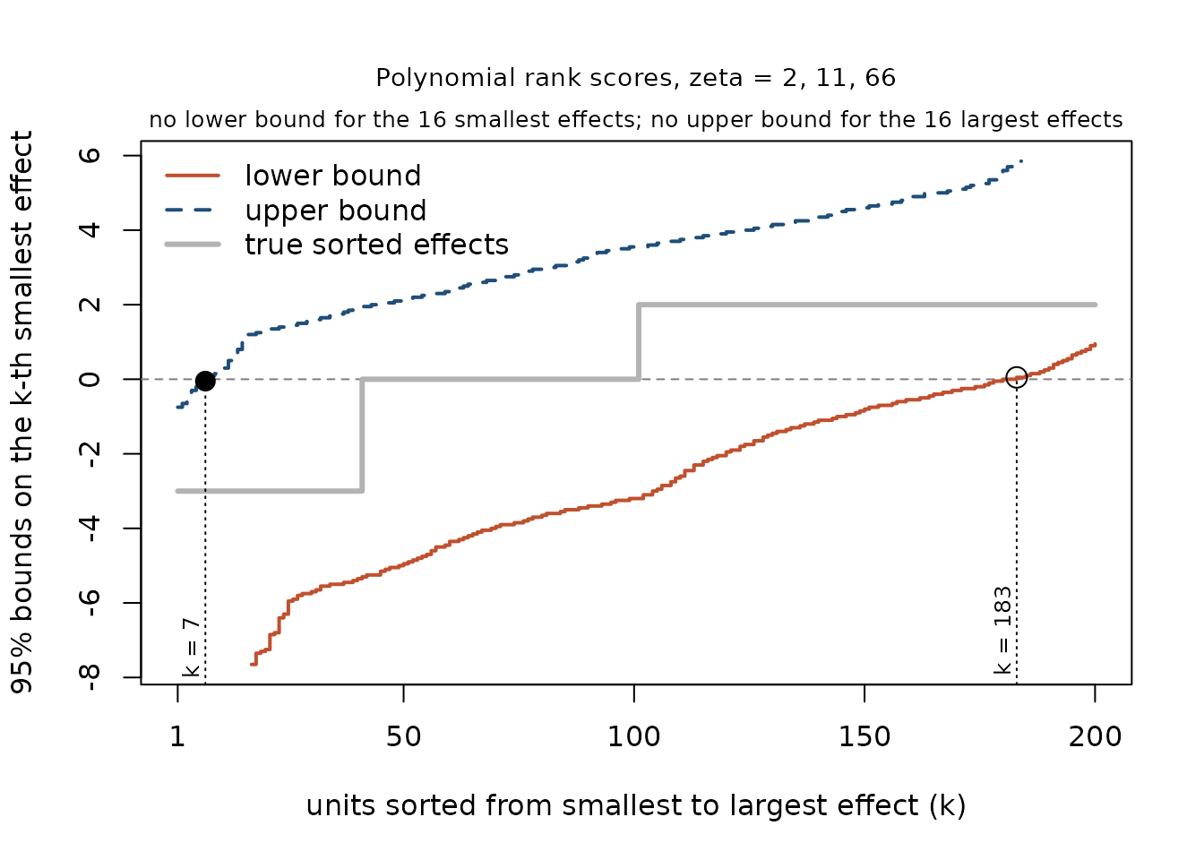
Four readings of the plot, each with the arithmetic behind it:
- The open circle is at k = 183, where the lower bound first rises above 0. The effects at positions 183 through 200 are all above 0, so at least units were helped.
- The filled circle is at k = 7, the last position where the upper bound is below 0. The effects at positions 1 through 7 are all below 0, so at least 7 units were harmed.
- Between the circles, each interval from the solid line to the dashed line contains 0. For those 175 positions we cannot tell from these data whether the effect is positive, negative, or zero.
- The grey line is the true sorted effects. It is at for k = 1 to 40, at 0 for k = 41 to 100, and at 2 for k = 101 to 200. At every k it lies between the two bounds. The method is built so that in at least 95 of every 100 experiments like this one, every true effect lies between its bounds. In this experiment they all did.
The teacher professional-development experiment
The electric_teachers data come from an experiment with
233 elementary school teachers in 7 sites. Within each site, the
researchers assigned teachers at random to one of three versions of a
professional development program in science or to a control group. The
variable TxAny is 1 for the 164 teachers assigned to any
version of the program and 0 for the 69 in the control group. The
outcome gain is a teacher’s score on a test of knowledge
about electric circuits after the program minus the score before it, in
percentage points.
Because the researchers randomized within sites, our analysis
compares teachers only with other teachers in their own site. We tell
cmrss() the sites by writing | Site in the
formula. Computing bounds within sites requires an optimization solver,
such as the one in the highs package. As in the simulation,
we compute the helped and harmed counts at alpha = 0.025
each.
data(electric_teachers)
t_helped <- cmrss(gain ~ TxAny | Site, data = electric_teachers,
                  set = "all", alpha = 0.025, nperm = nperm, tol = tol,
                  opt.method = "ILP_highs")
#> Warning in cmrss(gain ~ TxAny | Site, data = electric_teachers, set = "all", :
#> 29 of 233 units (12 percent) share the outcome value 10. Tied outcomes are
#> ranked by their order in the data, so reordering the rows can change p-values
#> and confidence bounds (see https://github.com/davidk91919/CMRSS/issues/5).
t_harmed <- cmrss(-gain ~ TxAny | Site, data = electric_teachers,
                  set = "all", alpha = 0.025, nperm = nperm, tol = tol,
                  opt.method = "ILP_highs")
#> Warning in cmrss(-gain ~ TxAny | Site, data = electric_teachers, set = "all", :
#> 29 of 233 units (12 percent) share the outcome value -10. Tied outcomes are
#> ranked by their order in the data, so reordering the rows can change p-values
#> and confidence bounds (see https://github.com/davidk91919/CMRSS/issues/5).
t_helped
#> cmrss: block-randomized experiment, 233 units, 164 treated
#> Polynomial scores with parameters 2, 11, 59; 1000 simulated assignments
#> With 97.5 percent confidence, at least 63 of 233 units have effects on gain above 0.
t_harmed
#> cmrss: block-randomized experiment, 233 units, 164 treated
#> Polynomial scores with parameters 2, 11, 59; 1000 simulated assignments
#> With 97.5 percent confidence, at least 0 of 233 units have effects on -gain above 0.
t_n_helped <- sum(t_helped$bounds$lower > 0)
t_n_harmed <- sum(t_harmed$bounds$lower > 0)
Both calls warn that 29 of the 233 teachers share a single value of
gain. cmrss() ranks tied outcomes by their
order in the data frame. With this many ties, a different order of the
rows could give somewhat different bounds.
With 95 percent confidence, at least 63 teachers gained from the
program. Analyzing -gain, we cannot show that any teacher
was harmed. A failure to show harm is not evidence that no teacher was
harmed. From the analysis of gain, as many as 233 - 63 =
170 teachers could have been harmed.
The same plot for the teachers, analyzed within sites, shows which sorted effects we can place above or below 0. These analyses also used the default polynomial rank scores, here with zeta = 2, 11, 59.
t_lower <- t_helped$bounds$lower
t_upper <- -rev(t_harmed$bounds$lower)
k_example <- 200
t_marks <- plot_bounds(t_lower, t_upper, unit = "teachers", zeta = t_helped$s,
                       mark_k = k_example,
                       ylab = "95% bounds on the k-th smallest effect on gain")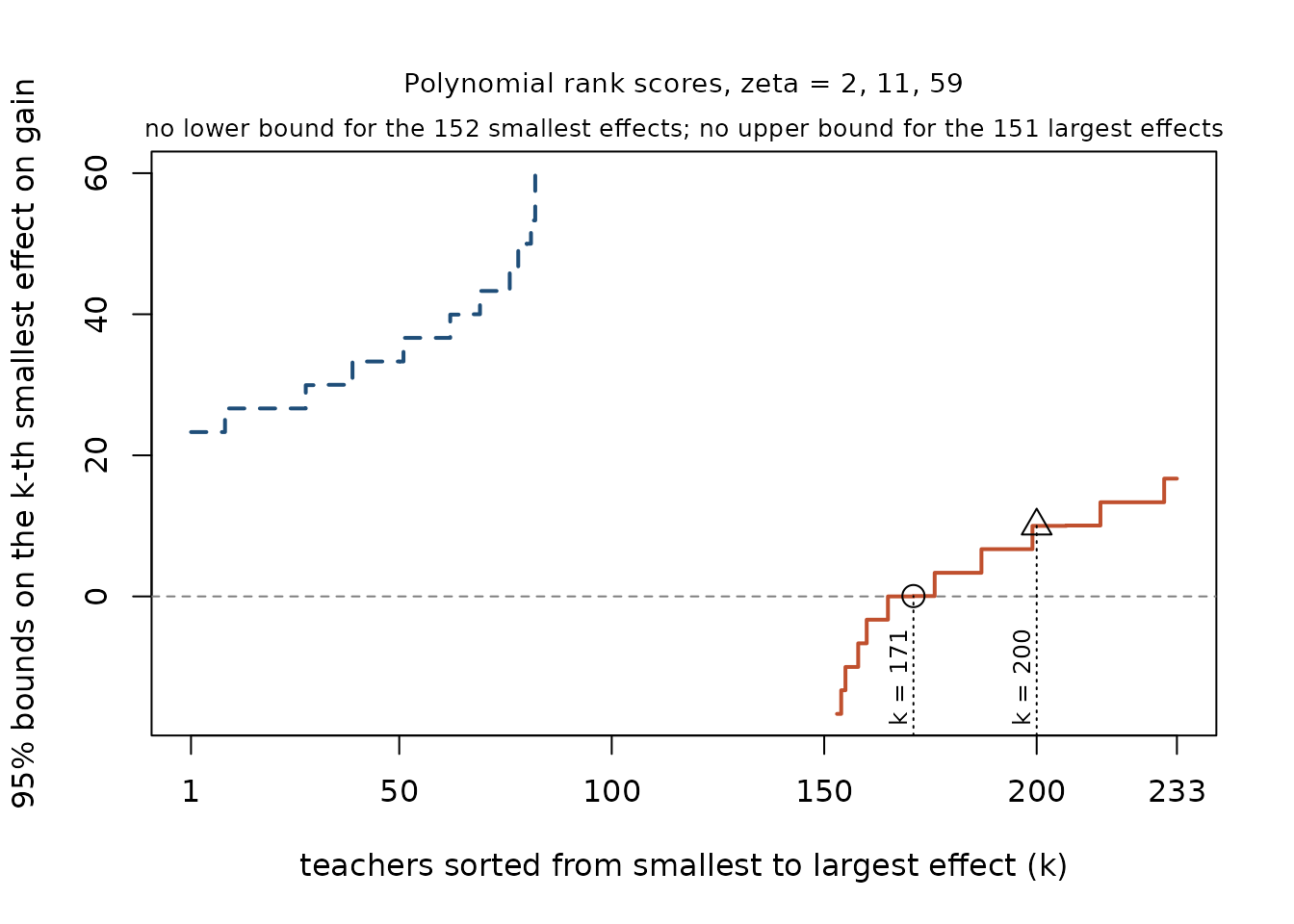
The open circle is at k = 171. The lower bound first rises above 0 there, so at least 233 - 171 + 1 = 63 teachers (27 percent) gained from the program. The bound also says how much they gained. The triangle is at k = 200. There the lower bound is 10 points, so the 200th smallest effect is at least 10 points. The effects at positions 200 through 233 are each at least as large as the 200th, so at least 233 - 200 + 1 = 34 teachers gained at least that much. No upper bound is below 0, so there is no filled circle: we cannot place any teacher’s effect below 0.
A p-value for the hypothesis that no one was harmed
Sometimes we want a single test rather than a count: could the data
have arisen if no unit was harmed? No unit was harmed when every effect
on
is at least 0. Then every effect on
is at most 0, and in particular the largest effect on
,
,
is at most 0. So the null hypothesis “no one was harmed” is the
hypothesis that the largest effect on
is at most 0. In cmrss() the largest effect is
quantile = 1, and the threshold is c = 0:
no_harm <- cmrss(-y ~ z, data = sim, quantile = 1, c = 0, set = "all",
                 nperm = nperm, tol = tol)
no_harm$test
#> $k
#> [1] 200
#>
#> $c
#> [1] 0
#>
#> $p.value
#> [1] 0
Many patterns of effects satisfy this null hypothesis. The test
computes its p-value under the pattern that makes harm hardest to
detect, in which no unit’s outcome changes at all. That p-value is
therefore valid for every pattern in which no one was harmed. With
set = "all", cmrss() tests the treated and the
control units separately and doubles the smaller of the two p-values,
for the same reason the counts above halved alpha.
None of the 1000 simulated random assignments produced a test statistic as large as the observed one, so the p-value is below 1/1000 = 0.001. (cmrss() reports such a p-value as 0.) At the 5 percent level we reject the hypothesis that no one was harmed. That agrees with the counts above, where we found at least 7 harmed units.
For the teachers, analyzed within sites:
t_no_harm <- cmrss(-gain ~ TxAny | Site, data = electric_teachers,
                   quantile = 1, c = 0, set = "all", nperm = nperm,
                   tol = tol, opt.method = "ILP_highs")
#> Warning in cmrss(-gain ~ TxAny | Site, data = electric_teachers, quantile = 1,
#> : 29 of 233 units (12 percent) share the outcome value -10. Tied outcomes are
#> ranked by their order in the data, so reordering the rows can change p-values
#> and confidence bounds (see https://github.com/davidk91919/CMRSS/issues/5).
t_no_harm$test
#> $k
#> [1] 233
#>
#> $c
#> [1] 0
#>
#> $p.value
#> [1] 1
The p-value is 1. We do not reject the hypothesis that no teacher was harmed. That agrees with the plot, where no upper bound fell below 0. As before, a large p-value is not evidence that no teacher was harmed: from the analysis of gain, as many as 170 teachers could have been.
The same test with the package’s p-value functions
cmrss() calls the package’s p-value functions, and we
can call them directly. They need the treatment and outcome as vectors,
a list of rank statistics, and the position k of the effect being
tested. comb_p_val_cre() counts k over all n units, and the
hypothesis it tests concerns the treated units: at most n - k of them
have an effect above c. With k = n and c = 0 on
,
that is the hypothesis that no treated unit was harmed. If no unit was
harmed then no treated unit was harmed, so a small p-value here also
rejects the hypothesis that no unit was harmed.
zeta <- no_harm$s    # the default polynomial parameters cmrss() used
ml <- lapply(zeta, function(s) {
  list(name = "Polynomial", r = s, std = TRUE, scale = FALSE)
})
set.seed(5)
p_direct <- comb_p_val_cre(sim$z, -sim$y, k = n, c = 0, ml, nperm = nperm)
set.seed(5)
p_cmrss <- cmrss(-y ~ z, data = sim, quantile = 1, c = 0, set = "treat",
                 nperm = nperm, tol = tol)$test$p.value
c(comb_p_val_cre = p_direct, cmrss = p_cmrss)
#> comb_p_val_cre          cmrss
#>              0              0
The two p-values are equal because, with the same random seed, both
compute the same test. cmrss() with
set = "treat" calls comb_p_val_cre() with
exactly these arguments.
For a block-randomized experiment the function is
pval_comb_block(). It counts k over the treated units only,
so the largest treated effect is k = sum(Z), and it needs
one list of score specifications per block for each statistic.
d <- electric_teachers
n_sites <- length(unique(d$Site))
ml_sites <- lapply(t_no_harm$s, function(s) {
  lapply(seq_len(n_sites), function(b) {
    list(name = "Polynomial", r = s, std = TRUE, scale = FALSE)
  })
})
pval_comb_block(d$TxAny, -d$gain, k = sum(d$TxAny), c = 0,
                block = factor(d$Site), methods.list.all = ml_sites,
                null.max = nperm, opt.method = "ILP_highs")
#> Warning in pval_comb_block(d$TxAny, -d$gain, k = sum(d$TxAny), c = 0, block =
#> factor(d$Site), : 29 of 233 units (12 percent) share the outcome value -10.
#> Tied outcomes are ranked by their order in the data, so reordering the rows can
#> change p-values and confidence bounds (see
#> https://github.com/davidk91919/CMRSS/issues/5).
#>   p.value test.stat
#>  1.000000 -4.168928
The result gives the p-value and the observed test statistic. The
p-value of 1 agrees with the result from cmrss() above.
set = "treat" in place of set = "all" tests
the narrower hypothesis that no treated unit was harmed. A test at a
single alpha stands on its own; the halving of
alpha used for the counts applies only when two statements
are reported together.
Choices that change the answer
With the argument set, we choose whose effects are
bounded: "treat", "control", or
"all".
With alpha, we choose the confidence level, 1 -
alpha. When we report the helped and harmed counts
together, we compute each at alpha / 2.
With s, we choose the rank statistics that
cmrss() combines. For polynomial scores the paper behind
this package calls these parameters zeta, and the plot titles above use
that name. A rank statistic replaces each outcome by its rank and adds
up a score for the rank of every treated unit. By default
cmrss() uses polynomial scores: the unit at rank r among n,
counting from the smallest outcome, gets the score
.
With s = 2 the score is proportional to the rank, so every rank counts.
With a large s nearly all the score sits on the few largest outcomes.
With a small s the combined test has more power against effects shared
by most units. With a large s it has more power against large effects in
a few units. The default combines three values of s, from 2 up to a
maximum set by the numbers of treated and control units. In the
simulation above they were 2, 11, 66. The section “Choosing s” in
?cmrss gives the rule, the simulations behind it, and the
alternative Stephenson scores (scores = "stephenson").
The method is built for outcomes that take many different values.
With a binary outcome, every observed outcome is 0 or 1, so each unit is
tied with every other unit that has the same value. The order of the
rows then decides most of the ranks, and cmrss() warns.
Every individual effect is also
,
,
or
,
so a bound can say little more than whether an effect is at least 0 or
at least 1. With a binary outcome there are four kinds of unit:
,
,
and
(helped), and
and
(harmed). Methods built on the counts of these four kinds, such as those
of Rigdon and Hudgens (2015, Statistics in Medicine 34, doi:10.1002/sim.6384) and Li
and Ding (2016, Statistics in Medicine 35, doi:10.1002/sim.6924), give
exact confidence intervals for the average effect on a binary
outcome.