Chapter 3 Design based inference
Most policy evaluations using administrative data or surveys report the results of their studies using estimators and hypothesis tests. We briefly define each for clarity.
Estimators: Although we can never know the true causal effect of a new policy (see Chapter 1), we can choose a method that provides us a best guess. E.g.: “The average amount saved for retirement by people in the treatment group was $1000 more than the average amount in the control group, so our estimate of the average treatment effect is $1000.”
Hypothesis tests: We can also test the plausibility of a particular hunch or hypothesis. Commonly, in program evaluation we focus on plausibility of the null hypothesis of no effect. E.g.: “We can reject the null hypothesis of no effect at a significance level given an estimated p-value of .” Ideally, we want to provide evidence that it is sufficiently unlikely for our result to be an artifact of random noise alone. Confidence intervals can be used to summarize hypothesis tests, so we generally think of them as tests rather than estimators.
When we are asked why we used some method for calculating an average treatment effect, -value, or confidence interval, we often say that our statistical analysis choices are based on the design of our studies. When applied to randomized experiments, this principle can be written simply as: “analyze as you randomize.” We provide an example of this principle in practice below. The intuition is to model unexplained variation in the data as noise introduced by random treatment assignment.
This idea, often known as randomization based or design based inference, was proposed by two of the founders of modern statistics. Jerzy Neyman’s 1923 paper showed how to use randomization to learn about what we would currently call “average treatment effects” (Neyman 1923), and Ronald A. Fisher’s 1935 book showed how to use randomization to test hypotheses about what we would currently call “treatment effects” (Fisher 1935). We favor design based justifications because we know exactly how a study was designed—after all, we and our agency collaborators chose the sample size, experimental arms, and outcome data.
Of course, there are other ways to justify statistical procedures, too. It is standard for researchers in many applied fields to instead motivate their tests using the idea of sampling from a larger (possibly infinite) population. This approach is more likely to depend on theoretical models of an estimator’s behavior as sample size increases indefinitely (“asymptotic” theory). OES projects frequently employ sampling-justified procedures as well. Importantly, some common procedures like the calculation of HC2 standard errors (discussed below) can be justified under either design based or sampling based statistical inference.
3.1 An example using simulated data
Imagine we have a simple randomized experiment where the relationship between outcomes and treatment is shown in Figure 3.1 (we illustrate the first 6 rows in the table below). Notice that, in this simulated experiment, the treatment changes the variability of the outcome in the treated group — this is a common pattern when the control group is a status quo policy.
## Read in data for the fake experiment.
dat1 <- read.csv("dat1.csv")

## Table of the first few observations.
knitr::kable(head(dat1[, c(1, 23:27)]))
** Read in data for the fake experiment.
import delimited using "dat1.csv", clear
rename v1 x
** Table of the first few observations.
list x y0 y1 z y id in 1/6, sep(6)| X | y0 | y1 | Z | Y | id |
|---|---|---|---|---|---|
| 1 | 0.000 | 6.123 | 0 | 0.000 | 1 |
| 2 | 0.000 | 2.741 | 0 | 0.000 | 2 |
| 3 | 0.000 | 7.215 | 0 | 0.000 | 3 |
| 4 | 2.056 | 6.708 | 0 | 2.056 | 4 |
| 5 | 0.000 | 5.654 | 1 | 5.654 | 5 |
| 6 | 10.409 | 15.561 | 0 | 10.409 | 6 |
## y0 and y1 are the true underlying potential outcomes.
with(dat1, {boxplot(list(y0,y1), names=c("Control","Treatment"), ylab="Outcomes")
stripchart(list(y0,y1), add=TRUE, vertical=TRUE)
stripchart(list(mean(y0), mean(y1)), add=TRUE, vertical=TRUE, pch=19, cex=2)})
** y0 and y1 are the true underlying potential outcomes.
label var y0 "Control"
label var y1 "Treatment"
* ssc install stripplot
stripplot y0 y1, box vertical iqr whiskers(recast(rcap)) ytitle("Outcomes") variablelabels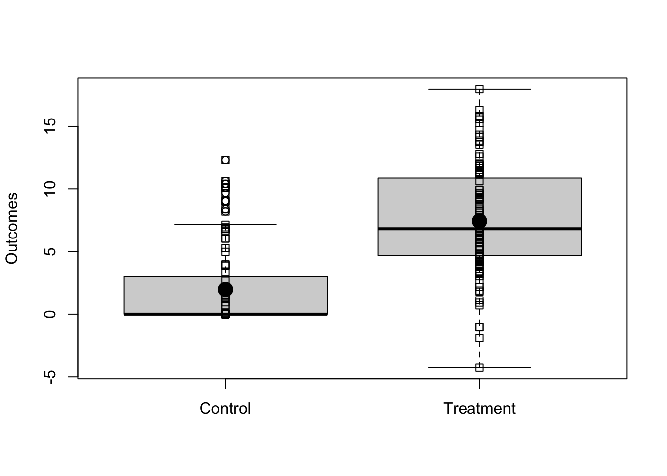
Figure 3.1: Simulated Experimental Outcomes
In this simulated data, we know the true average treatment effect (ATE) because we know both of the underlying true potential outcomes. The control potential outcome, , is written in the code as y0, meaning “the response person would provide if he/she were in the status quo or control group”. The treatment potential outcome, , is written in the code as y1, meaning “the response person would provide if he/she were in the new policy or treatment group.” We use to refer to the experimental arm. In this case for people in the status quo group and for people in the new policy group. The true treatment effect for each person is then the difference between that person’s potential outcomes under each treatment condition.
trueATE <- with(dat1, mean(y1) - mean(y0))
trueATE
qui tabstat y0 y1, stat(mean) save
global trueATE = r(StatTotal)[1,2] - r(StatTotal)[1,1][1] 5.453At this point, we have one realized experiment (defined by randomly assigning half of the people to treatment and half to control). The observed difference of means of the outcome, , between treated and control groups is an unbiased estimator of the true ATE, or the true “average treatment effect” (by virtue of random assignment to treatment).4 We can calculate this in a few ways: we can just calculate the difference of means, or we can take advantage of the fact that an ordinary least squares linear regression produces the same estimate when the explanatory variable is a binary treatment indicator.
estATE1 <- with(dat1, mean(Y[Z==1]) - mean(Y[Z==0]))
estATE2 <- lm(Y~Z, data=dat1)$coef[["Z"]]
c(estimatedATEv1=estATE1, estimatedATEv2=estATE2)
stopifnot(all.equal(estATE1, estATE2))
qui ttest y, by(z)
global estATE1 = round(r(mu_2) - r(mu_1), 0.001)
qui reg y z
global estATE2 = round(r(table)[1,1], 0.001)
di "estimatedATEv1=$estATE1 estimatedATEv2=$estATE2"
assert $estATE1 == $estATE2estimatedATEv1 estimatedATEv2
4.637 4.637 3.1.1 Randomization-based standard errors
How much would these estimates of the average treatment effect vary due to “random noise” if we repeated an experiment on the same group of people multiple times, randomly re-assigning treatment each time? The standard error of an estimate of the average treatment effect is one answer to this question. As the expected variation due to random noise gets larger relative to the size of our treatment effect estimate, we should become increasingly cautious about the risk that our finding is actually an artifact of random noise.5
Below, we simulate a simple experiment to help provide more intuition about what the standard error captures. We randomly re-assign treatment many times, save the resulting treatment effect estimates from each re-randomization, and calculate the standard deviation across them. This provides information about how far we should expect any one re-randomized treatment effect estimate to be from their mean.
## A function to re-assign treatment and recalculate the difference of means.
## Treatment was assigned without blocking or other structure, so we
## just permute or shuffle the existing treatment assignment vector.
simEstAte <- function(Z,y1,y0){
    Znew <- sample(Z)
    Y <- Znew * y1 + (1-Znew) * y0
    estate <- mean(Y[Znew == 1]) - mean(Y[Znew == 0])
    return(estate)
}

## Set up and perform the simulation
sims <- 10000
set.seed(12345)
simpleResults <- with(dat1,replicate(sims,simEstAte(Z = Z,y1 = y1,y0 = y0)))
seEstATEsim <- sd(simpleResults)

## The standard error of this estimate of the ATE (via simulation)
seEstATEsim
** A program to re-assign treatment and recalculate the difference of means.
** Treatment was assigned without blocking or other structure, so we
** just permute or shuffle the existing treatment assignment vector.
capture program drop simEstAte
program define simEstAte, rclass sortpreserve
version 18.0
syntax varlist(min=1 max=1), ///
control_outcome(varname) treat_outcome(varname)
qui sum `varlist' // Get # treated units
local numtreat = r(sum)
tempvar rand // Randomly sort (temporary var)
qui gen `rand' = runiform()
sort `rand'
tempvar Znew // New treatment
qui gen `Znew' = 0
qui replace `Znew' = 1 in 1/`numtreat'
tempvar Ynew // New revealed outcome
qui gen `Ynew' = (`Znew' * `treat_outcome') + ((1 - `Znew') * `control_outcome')
qui ttest `Ynew', by(`Znew')
return scalar estate = r(mu_2) - r(mu_1)
end
** Set up and perform the simulation
global sims 10000
set seed 12345
preserve
qui simulate estate = r(estate), reps($sims): simEstAte z, control_outcome(y0) treat_outcome(y1)
qui sum estate
global seEstATEsim = r(sd)
restore
** The standard error of this estimate of the ATE (via simulation)
di "$seEstATEsim"[1] 0.9256While this is useful for illustration, we do not need to rely on simulation to estimate design based standard errors. Gerber and Green (2012) and Dunning (2012) walk through the following expression for a feasible design based standard error of an average treatment effect estimate (e.g., a simple difference in means based on randomly assigned treatment). It’s called a “feasible” standard error because although it’s not exactly the same as the true design based standard error, it’s an approximation that we can calculate with a real sample. If we write as the set of all treated units and as the set of all non-treated units, we then have:
where is the sample variance such that .
In contrast, we cannot generally calculate the true design based standard error using a simple expression like this. I.e., we generally cannot apply a straightforward equation to a realized dataset and calculate exactly how far, on average, any re-randomized ATE will be from the mean across possible randomizations. There is a known expression for this (and you can see it in our code below)! However, it depends on the covariance between each unit’s potential outcomes, which is unobservable in real data. We can calculate this in our example for illustration, though, since we generated the data ourselves.
To make up for this, the feasible SE is derived to be greater than or equal to (but not smaller than) the true standard error on average. It is intentionally conservative. To illustrate these different calculation methods, we can compare the results of our simulation above to those of the feasible standard error expression. And we can also compare both to the true standard error.
We already have the simulated SE from the code above. Next, let’s calculate the true SE.
## True SE (Dunning Chap 6, Gerber and Green Chap 3, or Freedman, Pisani and Purves A-32).
## Requires knowing the true covariance between potential outcomes.
N <- nrow(dat1)
V <- var(cbind(dat1$y0,dat1$y1))
varc <- V[1,1]
vart <- V[2,2]
covtc <- V[1,2]
nt <- sum(dat1$Z)
nc <- N-nt

## Gerber and Green, p.57, equation (3.4)
varestATE <- (((varc * nt) / nc) + ((vart * nc) / nt) + (2 * covtc)) / (N - 1)
seEstATETrue <- sqrt(varestATE)
** True SE (Dunning Chap 6, Gerber and Green Chap 3, or Freedman, Pisani and Purves A-32).
** Requires knowing the true covariance between potential outcomes.
qui count
local N = r(N)
qui cor y0 y1, cov
local varc = r(C)[1,1]
local vart = r(C)[2,2]
local covtc = r(C)[1,2]
qui sum z
local nt = r(sum)
local nc = `N' - `nt'
** Gerber and Green, p.57, equation (3.4)
local varestATE = (((`varc' * `nt') / `nc') + ((`vart' * `nc') / `nt') + (2 * `covtc')) / (`N' - 1)
global seEstATETrue = sqrt(`varestATE')Then, let’s calculate the feasible standard error.
## Feasible SE
varYc <- with(dat1,var(Y[Z == 0]))
varYt <- with(dat1,var(Y[Z == 1]))
fvarestATE <- (N/(N-1)) * ( (varYt/nt) + (varYc/nc) )
estSEEstATE <- sqrt(fvarestATE)
** Feasible SE
qui sum y if z == 0
local varYc = r(sd) * r(sd)
qui sum y if z == 1
local varYt = r(sd) * r(sd)
local fvarestATE = (`N'/(`N'-1)) * ( (`varYt'/`nt') + (`varYc'/`nc') )
global estSEEstATE = sqrt(`fvarestATE')Importantly, this feasible design-based SE is not equivalent the standard error OLS regression provides by default. Among other things, default OLS SES are calculated under an iid errors assumption (“identically and independently distributed”). The feasible SE relaxes the “identically” part. Let’s record the OLS SE for illustration.
## OLS SE
lm1 <- lm(Y~Z, data=dat1)
iidSE <-  sqrt(diag(vcov(lm1)))[["Z"]]
** OLS SE
qui reg y z
global iidSE = _se[z] // Or: sqrt(e(V)["z","z"])Finally, we’ll calculate one more alternative called the HC2 standard error, which (Lin 2013) shows to be a design based SE for treatment effects estimated via OLS regression, potentially including additional control variables. I.e., it is an alternative to the feasible expression above, and one that can be easily computed for OLS coefficients using standard statistical software. Like the feasible SE in our expression above (which is specifically for a difference in means without any covariate adjustment), HC2 errors for an OLS coefficient should be conservative relative to the true SE. Note that under a sampling based approach to inference, the HC2 standard errors can instead be justified as a way of relaxing the assumption of “identically” distributed errors across. In other words, it is robust to a problem called “heteroscedasticity,” or “heteroscedasticity-consistent” (hence the HC in its name).
## HC2
HC2SE <- sqrt(diag(vcovHC(lm1, type = "HC2")))[["Z"]]
** HC2
qui reg y z, vce(hc2)
global HC2SE = _se[z] // Or: sqrt(e(V)["z","z"])All those SE estimates in hand, let’s review differences between the true standard error, the feasible standard error, the HC2 standard error, the standard error arising from direct repetition of the experiment, and the OLS standard error.
The HC2 OLS SE is intended to be conservative relative to the true SE (at least as large or larger on average). This is the case in our example. HC2 is similar to the feasible SE outlined above, and both are larger than the true SE. We also illustrate the accuracy of our earlier SE simulation as a way of thinking more intuitively about what the standard error represents. Lastly, recall that our design involves different outcome variances for the treated group and the control group. We would therefore expect what we are calling the OLS IID SE to be at least somewhat inaccurate (different variances across treatment groups means that errors are not “identically” distributed). However, as you can see below, this inaccuracy is still sometimes negligible in practice.
compareSEs <- c(simSE = seEstATEsim,
  feasibleSE = estSEEstATE,
  trueSE = seEstATETrue,
  olsIIDSE = iidSE,
  HC2SE = HC2SE)
sort(compareSEs)
matrix compareSEs = J(1, 5, .)
matrix compareSEs[1, 1] = $seEstATEsim
matrix compareSEs[1, 2] = $estSEEstATE
matrix compareSEs[1, 3] = $seEstATETrue
matrix compareSEs[1, 4] = $iidSE
matrix compareSEs[1, 5] = $HC2SE
matrix colnames compareSEs = "simSE" "feasibleSE" "trueSE" "olsIIDSE" "HC2SE"
matrix list compareSEs olsIIDSE trueSE simSE HC2SE feasibleSE
0.8930 0.9189 0.9256 1.0387 1.0439 To provide a more rigorous comparison of these SE estimation methods, the code chunk below defines a function to calculate an average treatment effect, the OLS iid SE, and the OLS HC2 SE. It then uses this function to calculate SEs for random permutations of treatment 10000 times. Averaging across the simulated estimates provides a better illustration of their relative performance. As expected, the OLS IID SE now underestimates the true SE, while the HC2 SE is conservative as intended. The risk of underestimating the SE is that it could lead us to be overconfident when interpreting statistical findings.
## Define a function to calculate several SEs, given potential outcomes and treatment
sePerfFn <- function(Z,y1,y0){
    Znew <- sample(Z)
    Ynew <- Znew * y1 + (1-Znew) * y0
    lm1 <- lm(Ynew~Znew)
    olsIIDse <-  sqrt(diag(vcov(lm1)))[["Znew"]]
    HC2SE <- sqrt(diag(vcovHC(lm1,type = "HC2")))[["Znew"]]
    return(c(estATE=coef(lm1)[["Znew"]],
         olsIIDse=olsIIDse,
         HC2SE=HC2SE))
}

## Perform a simulation using this function
set.seed(12345)
sePerformance <- with(dat1, replicate(sims, sePerfFn(Z = Z, y1 = y1, y0 = y0)))
ExpectedSEs <- apply(sePerformance[c("olsIIDse", "HC2SE"),], 1, mean)
c(ExpectedSEs, trueSE=seEstATETrue, simSE=sd(sePerformance["estATE",]))
** Define a function to calculate several SEs, given potential outcomes and treatment
capture program drop sePerfFn
program define sePerfFn, rclass sortpreserve
version 18.0
syntax varlist(min=1 max=1), control_outcome(varname) treat_outcome(varname)
qui sum `varlist' // As in the program above
local numtreat = r(sum)
tempvar rand
qui gen `rand' = runiform()
sort `rand'
tempvar Znew
qui gen `Znew' = 0
qui replace `Znew' = 1 in 1/`numtreat'
tempvar Ynew
qui gen `Ynew' = (`Znew' * `treat_outcome') + ((1 - `Znew') * `control_outcome')
qui reg `Ynew' `Znew' // Regression now instead of ttest
local olsIIDSE = _se[`Znew']
qui reg `Ynew' `Znew', vce(hc2)
local HC2SE = _se[`Znew']
return scalar olsIIDSE = `olsIIDSE' // Prepare output
return scalar HC2SE = `HC2SE'
return scalar estATE = _b[`Znew']
end
** Perform a simulation using this function
set seed 12345
preserve
qui simulate ///
olsIIDSE = r(olsIIDSE) HC2SE = r(HC2SE) estATE = r(estATE), ///
reps($sims): ///
sePerfFn z, control_outcome(y0) treat_outcome(y1)
qui sum estATE
global simSE = r(sd)
qui sum olsIIDSE
global olsIIDSE = r(mean)
qui sum HC2SE
global HC2SE = r(mean)
restore
di "Expected IID SE: $olsIIDSE"
di "Expected Neyman SE: $HC2SE"
di "SIM SE: $simSE"
di "True SE: $seEstATETrue"olsIIDse HC2SE trueSE simSE
0.8511 0.9574 0.9189 0.9256 3.1.2 Randomization-based confidence intervals
When we have a large enough sample size in an RCT, we can estimate the ATE, calculate design based standard errors, and then use them to create large-sample justified confidence intervals through either of the following approaches. Though researchers using design based inference may often rely on manually simulating treatment many times to calculate a p-value (randomization inference, below), asymptotic approximations like those sampling based inference typically relies on (theoretical findings about an estimator’s behavior as sample size increases indefinitely) can be used in design based statistical inference as well.6 In fact, this is the setting in which (Lin 2013) shows that HC2 errors are a feasible design based standard error (HC2 errors may not be appropriately conservative if a sample is too small).
## The difference_in_means function comes from the estimatr package.
# (design based feasible errors by default)
estAndSE1 <- difference_in_means(Y ~ Z, data = dat1)

## Note that coeftest and coefci come from the lmtest package
# (narrower intervals due to a different d.o.f.)
est2 <- lm(Y ~ Z, data = dat1)
estAndSE2 <- coeftest(est2, vcov.=vcovHC(est2, type = "HC2"))
estAndCI2 <- coefci(est2, vcov.=vcovHC(est2, type = "HC2"), parm = "Z")

## Organize output
out <- rbind( unlist(estAndSE1[c(1,2,6:8)]),  c(estAndSE2[2,-3], estAndCI2) )
out <- apply(out, 2, round, 3)
colnames(out) <- c("Est", "SE", "pvalue", "CI lower", "CI upper")
row.names(out) <- c("Approach 1 (diff. means)", "Approach 2 (OLS)")
out
** Organize output
matrix compareCIs = J(2, 5, .)
matrix rownames compareCIs = "Approach 1 (diff. means)" "Approach 2 (OLS)"
matrix colnames compareCIs = "Est" "SE" "pvalue" "CI lower" "CI upper"
** A difference in means test assuming unequal variances
** (equivalent to the design-based estimator, as discussed above)
ttest y, by(z) unequal
local diffmeans = r(mu_2) - r(mu_1)
matrix compareCIs[1,1] = round(`diffmeans', 0.001)
matrix compareCIs[1,2] = round(r(se), 0.001)
matrix compareCIs[1,3] = round(r(p), 0.001)
matrix compareCIs[1,4] = round(`diffmeans' - (invttail(r(df_t), 0.025) * r(se)), 0.001)
matrix compareCIs[1,5] = round(`diffmeans' + (invttail(r(df_t), 0.025) * r(se)), 0.001)
** A regression-based approach (narrower intervals due to a different d.o.f)
reg y z, vce(hc2) // See: "matrix list r(table)"
matrix compareCIs[2,1] = round(r(table)[1, 1], 0.001)
matrix compareCIs[2,2] = round(r(table)[2, 1], 0.001)
matrix compareCIs[2,3] = round(r(table)[4, 1], 0.001)
matrix compareCIs[2,4] = round(r(table)[5, 1], 0.001)
matrix compareCIs[2,5] = round(r(table)[6, 1], 0.001)
matrix list compareCIs Est SE pvalue CI lower CI upper
Approach 1 (diff. means) 4.637 1.039 0 2.524 6.750
Approach 2 (OLS) 4.637 1.039 0 2.576 6.699Above, we mention something called “randomization inference.” This is an alternative approach to calculating p-values and performing a hypothesis test for randomized trials entirely through simulation (without calculating a standard error). It’s similar to the example we use to open this chapter. We can use randomization inference in a study any time treatment assignment itself was randomized. It may be appropriate even in samples that are too small to justify calculating standard errors based on large sample approximations. It also sometimes lets us sidestep tricky problems like choosing how to cluster errors when there is imperfect cluster level assignment (Abadie et al. 2023). Like bootstrapping (not currently discussed in this SOP), the core advantage of randomization inference is it’s flexibility to handle cases where there isn’t a clear or easy way to calculate analytical standard errors (i.e., based on an equation someone has already derived).
We talk about randomization inference more in Chapters 4 and 5 (with coded examples). But to provide a quick walk through here of the simplest version:
Start by estimating an ATE using your real data:
Randomly generate a new treatment variable, , using the exact same procedure you used to generate the first one (i.e., generate an alternative treatment assignment you could have used instead).
Estimate a treatment effect for this permuted treatment variable, . Save it.
Repeat that process many times, yielding a distribution of values.
Finally, to get a two-sided p-value, calculate the proportion of times the absolute value of any is greater than or equal to the absolute value of : .
Because this method doesn’t yield a standard error, we can’t calculate a confidence interval the same way we did above. But you can still estimate a confidence interval when using randomization inference! It’s just more involved. This is sometimes called an inverted hypothesis test:
Choose a “grid” of values to consider, , generally symmetric around 0 (e.g., [-0.5, 0.5]).
For each , construct a new outcome measure: , and estimate a treatment effect, . Then, calculate a p-value for using randomization inference:
Repeat the procedure we outline above, randomly permuting treatment many times and estimating a treatment effect on each time, comparing the simulated distribution of effects to to calculate a p-value.
This is your p-value for a given .
Finally, look at the p-values across all . The highest and lowest values of that yield p-values greater than 0.05 are our simulated 95% confidence interval.
## Define the grid to search through
grid <- seq(-10, 10, 0.05)

## Loop through values in this grid
res <- matrix(NA, length(grid), 2)
i <- 0
for (g in grid) {

  ## Update loop index
  i <- i + 1

  ## Create outcome for this g
  gdat <- dat1
  gdat$yg <- gdat$Y - g*gdat$Z

  ## "Real" treatment effect for this g
  mod <- lm(yg ~ Z, data = gdat)

  ## p-value through randomization inference
  ridraws <- lapply(
    1:500,
    function(.x) {
      gdat$Zri <- sample(gdat$Z, length(gdat$Z), replace = F)
      lm(yg ~ Zri, data = gdat)$coefficients[2]
      }
    )
  ridraws <- do.call(c, ridraws)
  res[i,1] <- g
  res[i,2] <- mean(abs(ridraws) >= abs(mod$coefficients[2]))

}

## Compute CI from results
res <- res[ res[,2] > 0.05, ]
c( min(res[,1]), max(res[,1]) )
** Define the grid to search through
numlist "-10(0.05)10"
local grid `r(numlist)'
macro list _grid
** Simple RI program to use here
capture program drop ri_p
program define ri_p, rclass
capture drop Zri
qui complete_ra Zri, m(25)
qui reg yg Zri
return scalar taur = _b[Zri]
end
** Loop through values in this grid
tempfile realdat
save `realdat', replace
local i = 0
foreach g of local grid {
local ++i
** Create outcome for this g
use `realdat', clear
qui gen yg = y - `g' * z
** Real regression for this g
qui reg yg z
local taug = _b[z]
** RI inference for this g
qui simulate taur = r(taur), ///
reps(500) : ///
ri_p
replace taur = abs(taur) >= abs(`taug')
collapse (mean) taur
qui gen g = `g'
** Save results
if `i' == 1 {
qui tempfile running
qui save `running'
}
else {
append using `running'
qui save `running', replace
}
** Return to original data
use `realdat', clear
}
** Load the results
use `running', clear
** Compute the CI
keep if taur > 0.05
qui sum g
global lower = r(min)
global upper = r(max)
di "$lower, $upper"[1] 2.85 6.35Notice that this CI is narrower than the other CIs above. This isn’t a coincidence. Standard statistical inference using large sample justified standard errors normally evaluates the compatibility of our data with the weak null hypothesis of no treatment effect on average. Randomization inference instead evaluates the compatibility of our data with the sharp null hypothesis of no effect at all for any unit. Especially in small samples, we might have more power against the sharp null than the weak null (policy relevance is also a factor in choosing the null that it is more interesting to evaluate). We discuss this again in Chapter 5.
3.2 Summary: What does a design based approach mean for policy evaluation?
Let’s review some important terms. Hypothesis tests produce -values telling us how much information we have against a null hypothesis. Estimators produce guesses about the size of some causal effect like the average treatment effect (i.e., “estimates”). Standard errors summarize how our estimates might vary from experiment to experiment by random chance, though we can only observe one experiment in practice. Confidence intervals tell us which ranges of null hypotheses are more versus less consistent with our data.
In the frequentist approach to probability (the only approach we consider in this SOP), the properties of both -values and standard errors arise from some process of repetition. Statistics textbooks often encourage us to imagine that this process of repetition involves repeated sampling from a larger (potentially infinite) population. But most OES work involves a pool of people who do not represent a well-defined population, nor do we tend to have a strong probability model of how these people and not others entered our sample. Instead, we have a known process of random assignment to an experimental intervention within a fixed sample. This often makes a randomization based approach to inference natural for our work, and helps our work be easiest to explain and interpret for our policy partners.
References
See https://egap.org/resource/10-types-of-treatment-effect-you-should-know-about/ for a demonstration that the difference-in-means between the observed treatment and control groups is an unbiased estimator of the average treatment effect itself, and what it means to be unbiased.↩︎
As discussed above, under a design based approach, random noise is assumed to be introduced by treatment assignment decisions. Under more common sampling-based inference procedures, it is instead assumed to be introduced by the process of sampling from a larger population.↩︎
Now, instead of imagining that we’re taking a larger and larger sample from the population, we’re imagining randomly assigning treatment in a bigger and bigger sample.↩︎